Let's get started
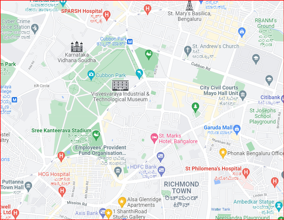
Look at a piece of Google Map.
What different objects do you see?
What information do you think went into making it?
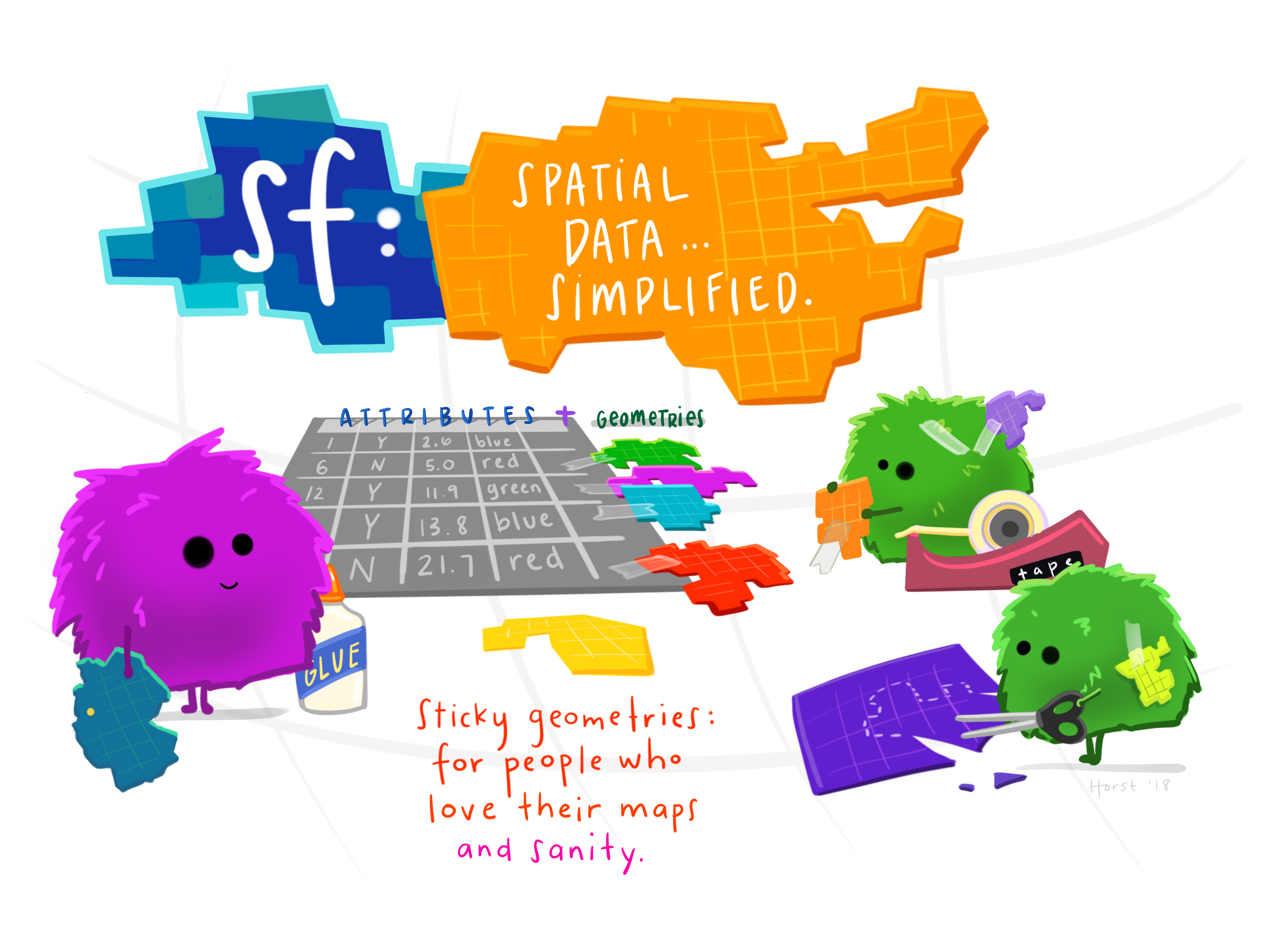
The picture shows a familiar looking data-frame with the far-right column containing geometries, or shapes....hmmm.
What is a Feature?
A Thing, or an Object in the real world
Examples of Features:
- A Tree or a Lamp-post
- A forest stand
- A city with building, streets, and parks
- A County or State
- A Country
- An Island

What is a Feature Geometry?
Features have a geometry describing where on Earth the feature is located
- Features = Shapes + Location Data
- The geometry of a tree can be the delineation of its crown ( Polygon )
- Of its stem, (Polygon )
- or the point indicating its centre. (Point )
- A feature geometry is called simple
- when it consists of points connected by straight line pieces,
- and does not intersect itself.
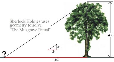
'Whose was it?'
'His who is gone.'
'Who shall have it?'
'He who will come.'
('What was the month?'
'The sixth from the first.')
'Where was the sun?'
'Over the oak.'
'Where was the shadow?'
'Under the elm.'
'How was it stepped?'
'North by ten and by ten, east by five and by five, south by two and by two, west by one and by one, and so under.'
'What shall we give for it?'
'All that is ours.'
'Why should we give it?'
'For the sake of the trust.'
So Finally, What is a Spatial Data Frame in R?
- Features Geometries + Attribute data in a single Data Frame
- Geometries give where the feature is located and its shape
- Attributes describe other properties:
- Tree height
- Flower or foliage colour
- Trunk diameter at breast height at a particular date,
- Tree species and so on.
Kinds of Geospatial Data
- Examples:
- Point: buildings, offices, venues, etc in a city
- LineString: Roads, rivers and railways
- Polygon: a lake, a golf course, or the border of a country
- MultiPolygon: Any non-contiguous set of areas, a set of suburbs for example
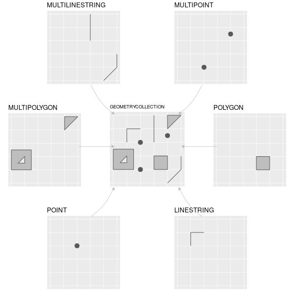
How are these shapes represented?
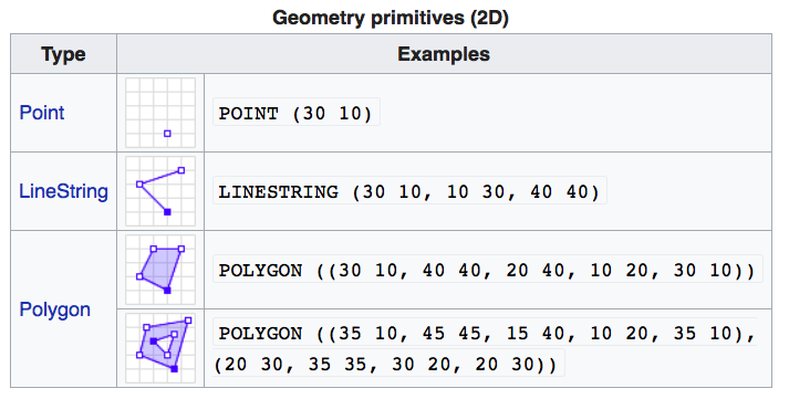
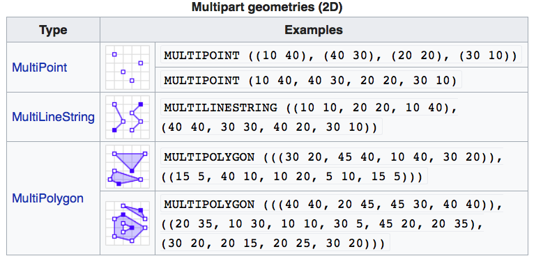
- These formulaic descriptions are called WKT: Well Known Text
lonlatpairs. NOT separated by comma!- Closed features have last point repeated
- Parentheses denotes shapes and nesting
- Note: Polygons can have "holes" in them!!
How are these shapes represented?
If we examine a spatial data fram in sf we get:
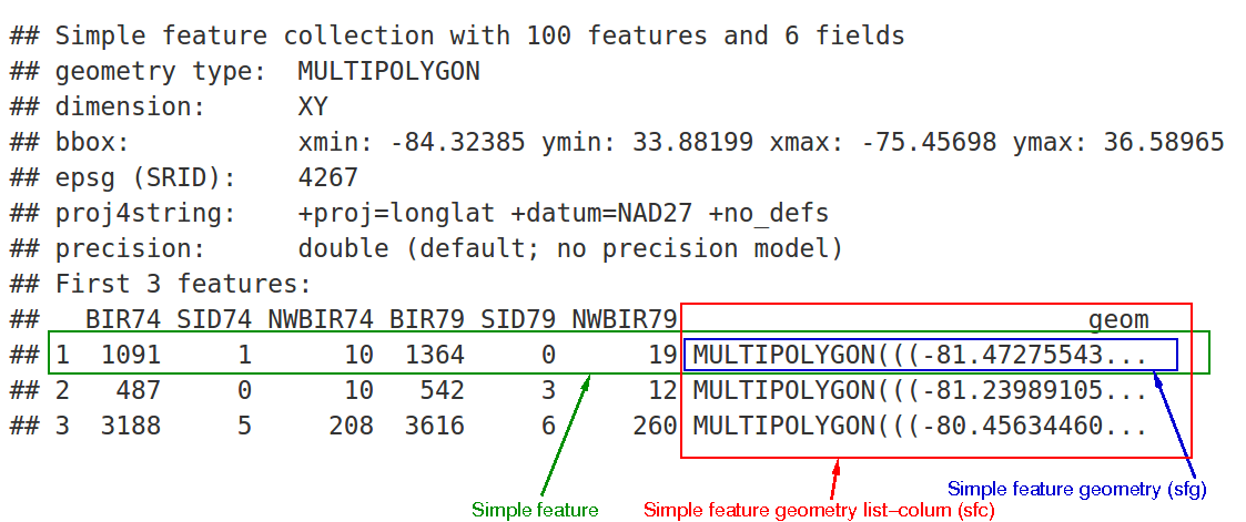
The sf : Spatial Data Frame: Point Geometry
# Let's get the India Boundarydata("world")india <- World %>% filter(iso_a3 == "IND")crs_india <- st_crs(india)points <- # Create 5 random points data.frame(lon = rnorm(5, 77, 2), lat = rnorm(5, 23, 5))#str(points) # Convert to spatial data framepoints_sf <- st_as_sf(points, coords = c("lon", "lat"), crs = crs_india)#str(points_sf)ggplot() + geom_sf(data = india) + geom_sf(data = points_sf, colour = "red", size = 4)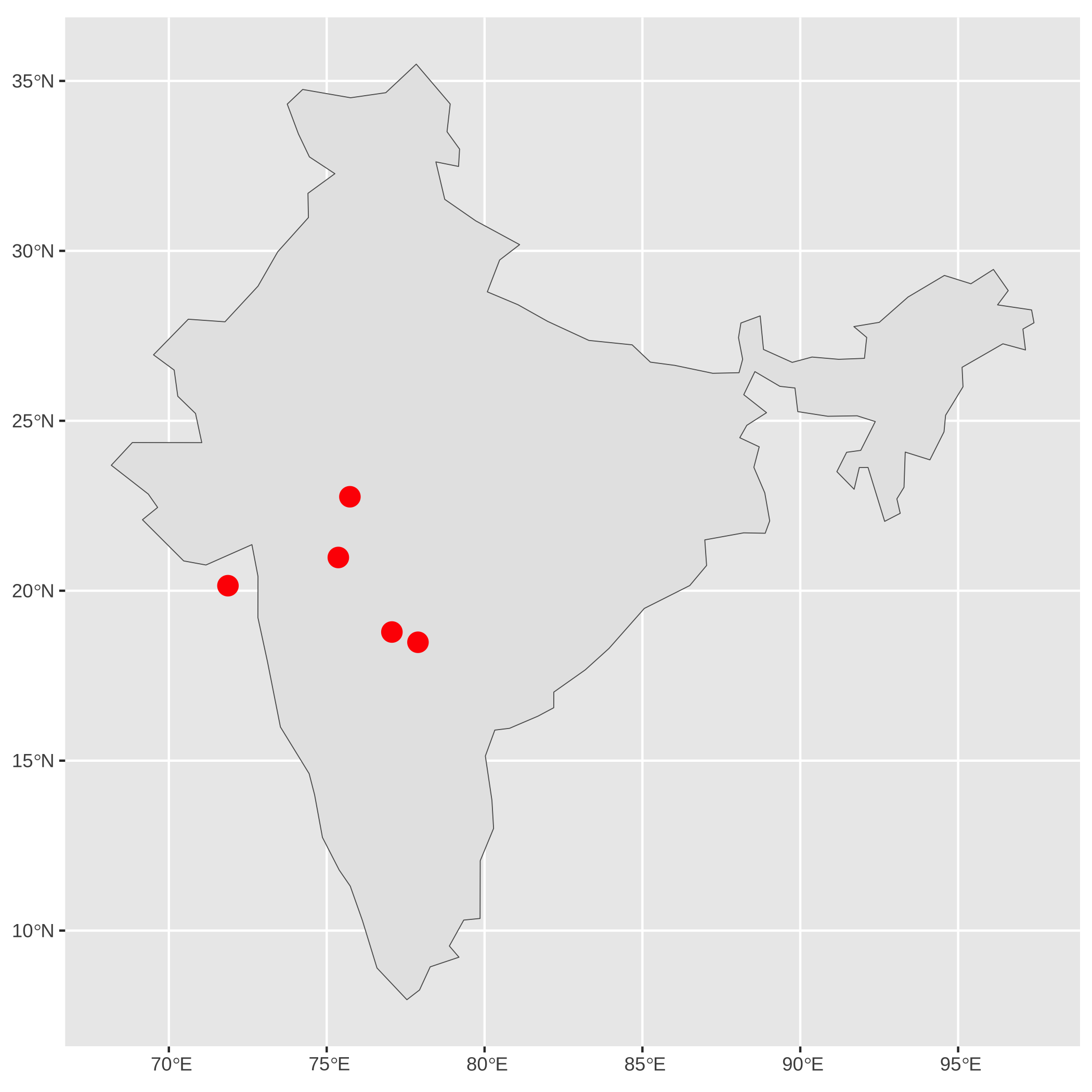
The sf:Spatial Data Frame: Polygon Geometry
# Let's create three SQUARES# (Using matrices)# Center them over Central India # (Lon: 77, Lat: 13)# outer <- matrix(c(0,0,10,0,10,10,0,10,0,0) + c(77,13), ncol=2, byrow=TRUE)hole1 <- matrix(c(1,1,1,2,2,2,2,1,1,1) + c(77,13),ncol=2, byrow=TRUE)hole2 <- matrix(c(5,5,5,6,6,6,6,5,5,5) + c(77,13),ncol=2, byrow=TRUE)# Now pile all matrices into a **LIST*pl1 <- list(outer, hole1, hole2)pl1_polygon <- st_polygon(pl1) %>% # feature geometry st_sfc() %>% # feature column st_as_sf(crs = crs_india) # spatial data frameggplot() + geom_sf(data = india) + geom_sf(data = pl1_polygon, colour = "red")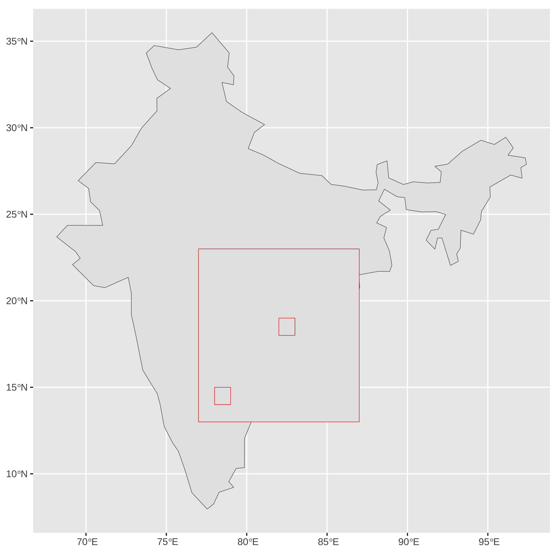
The sf:Spatial Data Frame: Multi-Polygon Geometry
[,1] [,2][1,] 77 13[2,] 87 13[3,] 87 23[4,] 77 23[5,] 77 13List of 3 $ : num [1:5, 1:2] 77 87 87 77 77 13 13 23 23 13 $ : num [1:5, 1:2] 78 78 79 79 78 14 15 15 14 14 $ : num [1:5, 1:2] 82 82 83 83 82 18 19 19 18 18pol1 <- list(outer, hole1, hole2)pol2 <- list(outer + 12, hole1 + 12)pol3 <- list(outer - 12)mp <- list(pol1,pol2,pol3)mp1 <- st_multipolygon(mp) %>% #feature geometry st_sfc() %>% #feature column st_as_sf(crs = crs_india) # sf dataframehead(mp1,3)ggplot() + geom_sf(data = india) + geom_sf(data = mp1, colour = "red")Simple feature collection with 1 feature and 0 fieldsGeometry type: MULTIPOLYGONDimension: XYBounding box: xmin: 65 ymin: 1 xmax: 99 ymax: 35Geodetic CRS: WGS 84 x1 MULTIPOLYGON (((77 13, 87 1...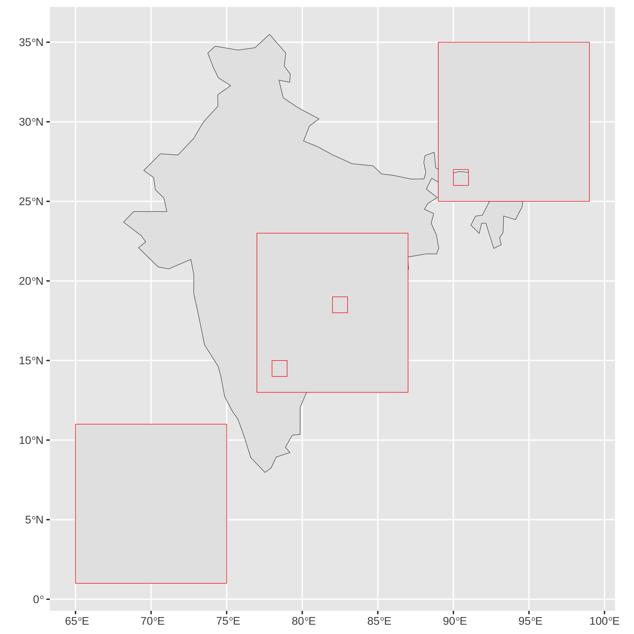
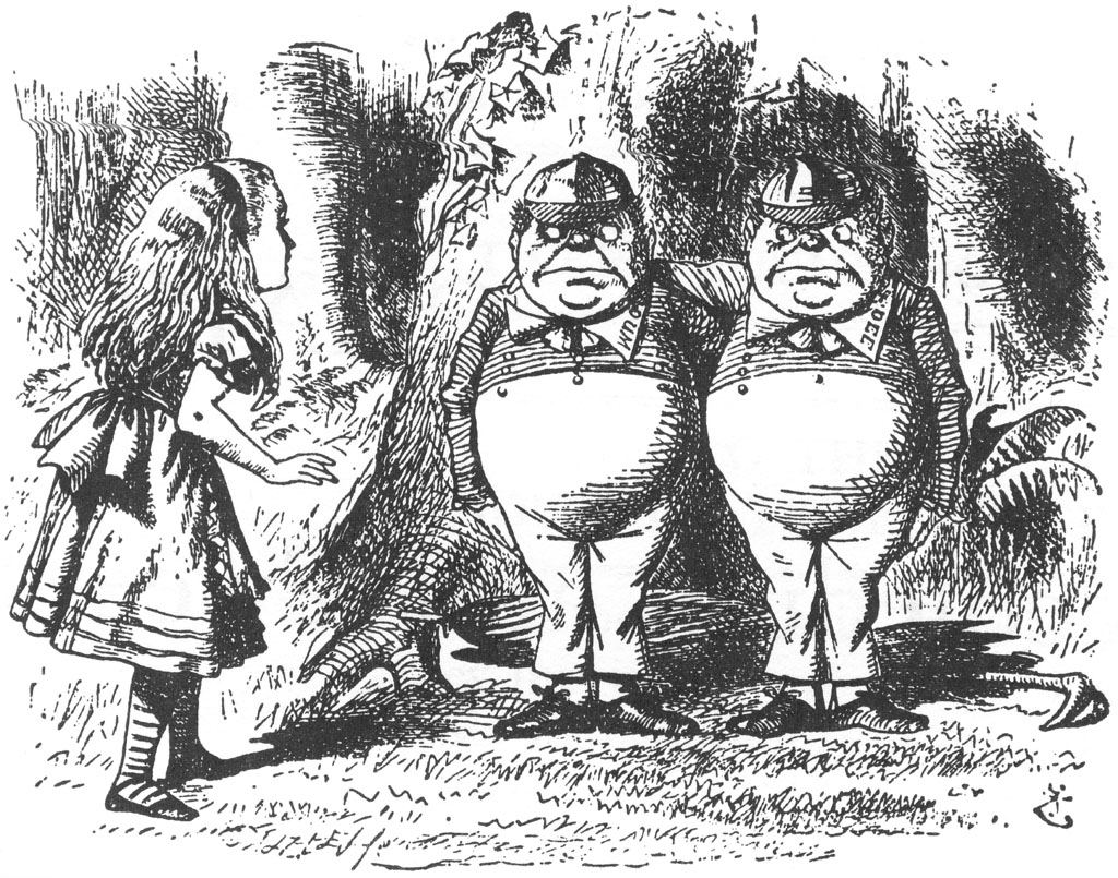
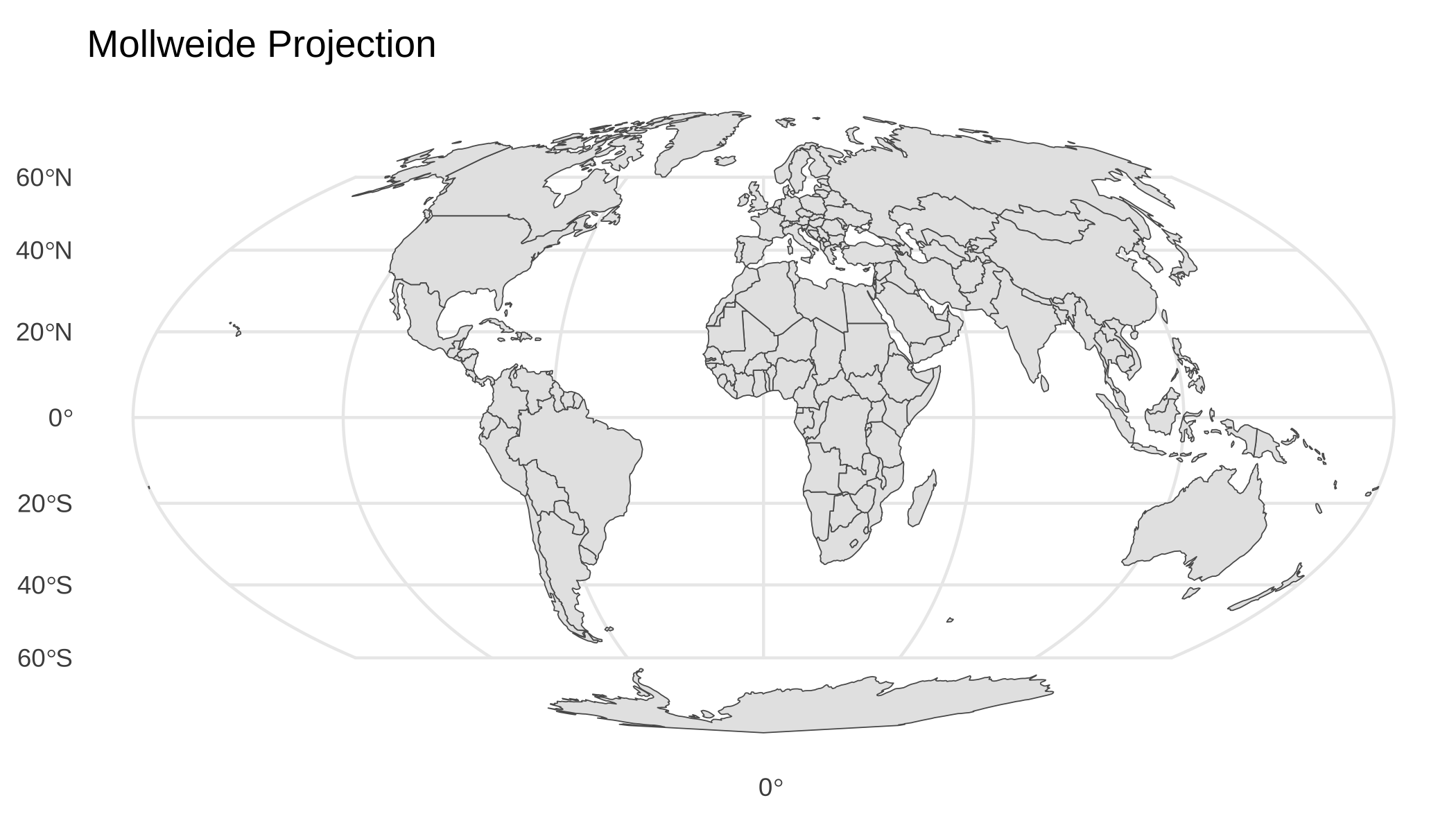
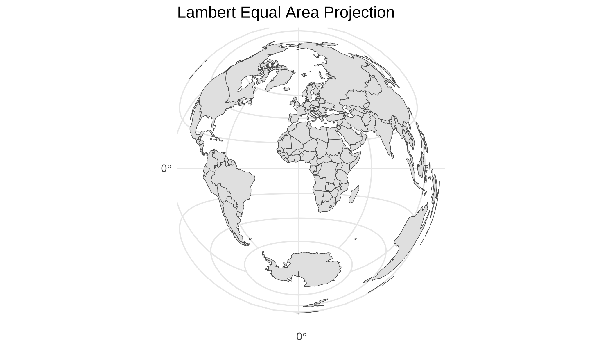
Map Projections: Through the Looking Glass
A Projection is a shadow or Image...
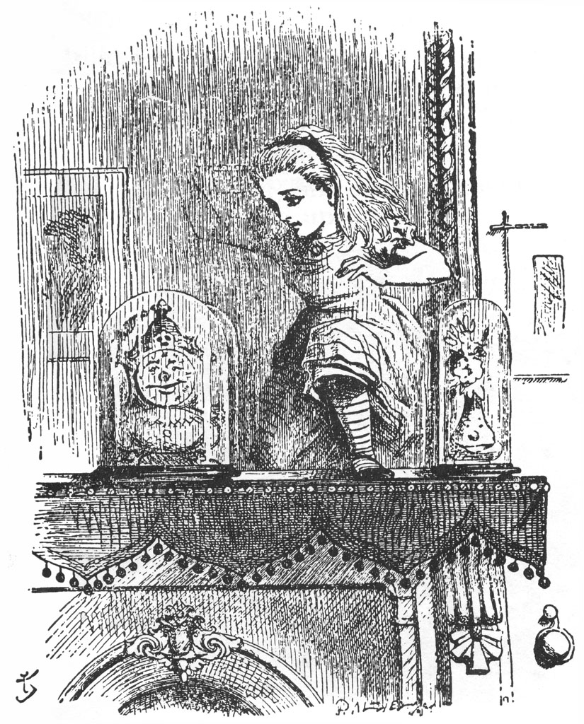
We see Maps Through The Looking Glass...
No Two Map Projections are Alike!
Why do we Need Projections?

- Cannot Flatten the Earth's Surface onto a 2D surface
- Just as we cannot flatten the Orange Peel
- So: we need Mirrors, Shadows and Images and Lights...just like Alice
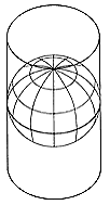
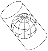
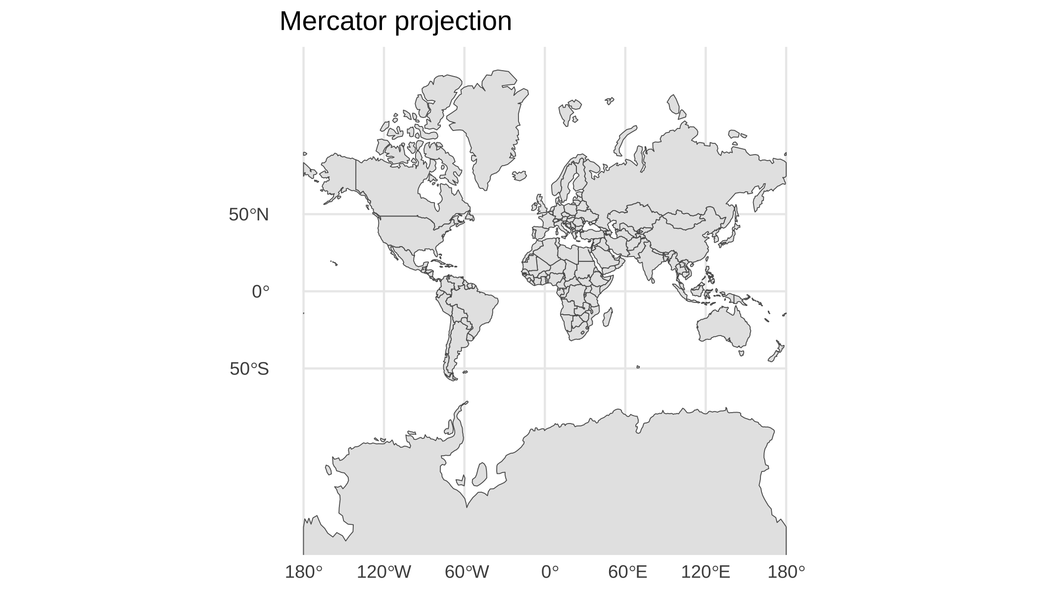
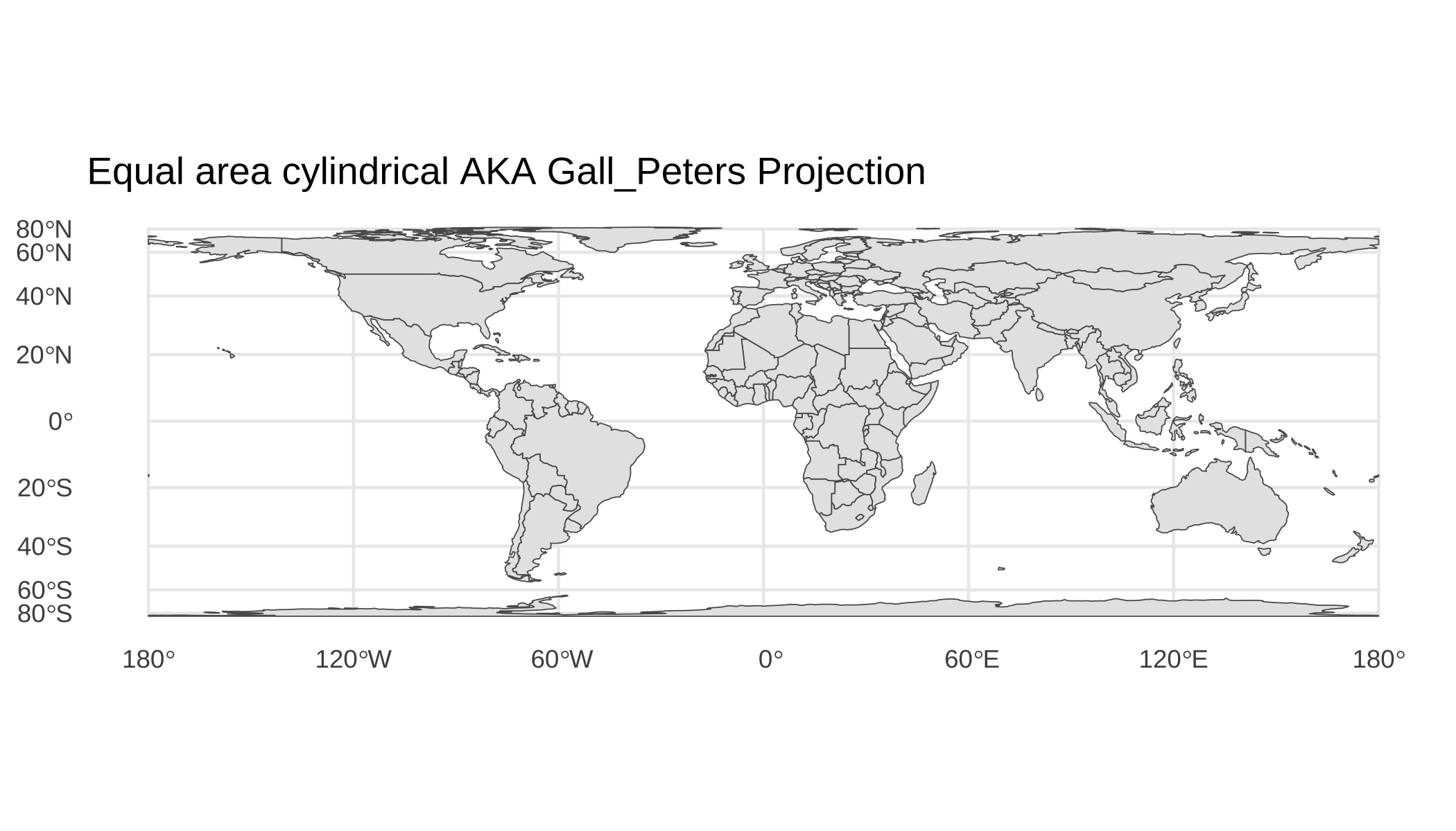
Cylindrical Projection
Regular Cylindrical Projection
Oblique Cylindrical Projection
Azimuthal Projection
Polar Azimuthal Projection
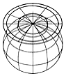
Oblique Azimuthal Projection
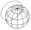
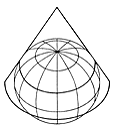
Conical Projection
Projections with coord_sf()
'data.frame': 5 obs. of 2 variables: $ lon: num 74.3 77.1 81.7 75.2 76.7 $ lat: num 27.04 9.47 20.1 20.28 26.21Let's create an Azimuthal Equal Area Projection in R. We can use the Lambert Azimuthal Equal-Area Projection:
ggplot() + geom_sf(data = world, crs = "+proj=laea +lat_0=23 +lon_0=77 +x_0=4321000 #<< +y_0=3210000 +ellps=GRS80 +units=m +no_defs") + geom_sf(data = india, crs = "+proj=laea +lat_0=23 +lon_0=77 +x_0=4321000 #<< +y_0=3210000 +ellps=GRS80 +units=m +no_defs") + geom_sf(data = points_sf, colour = "red", size = 2) + coord_sf(crs = "+proj=laea +lat_0=23 +lon_0=77 +x_0=4321000 +y_0=3210000 +ellps=GRS80 +units=m +no_defs" )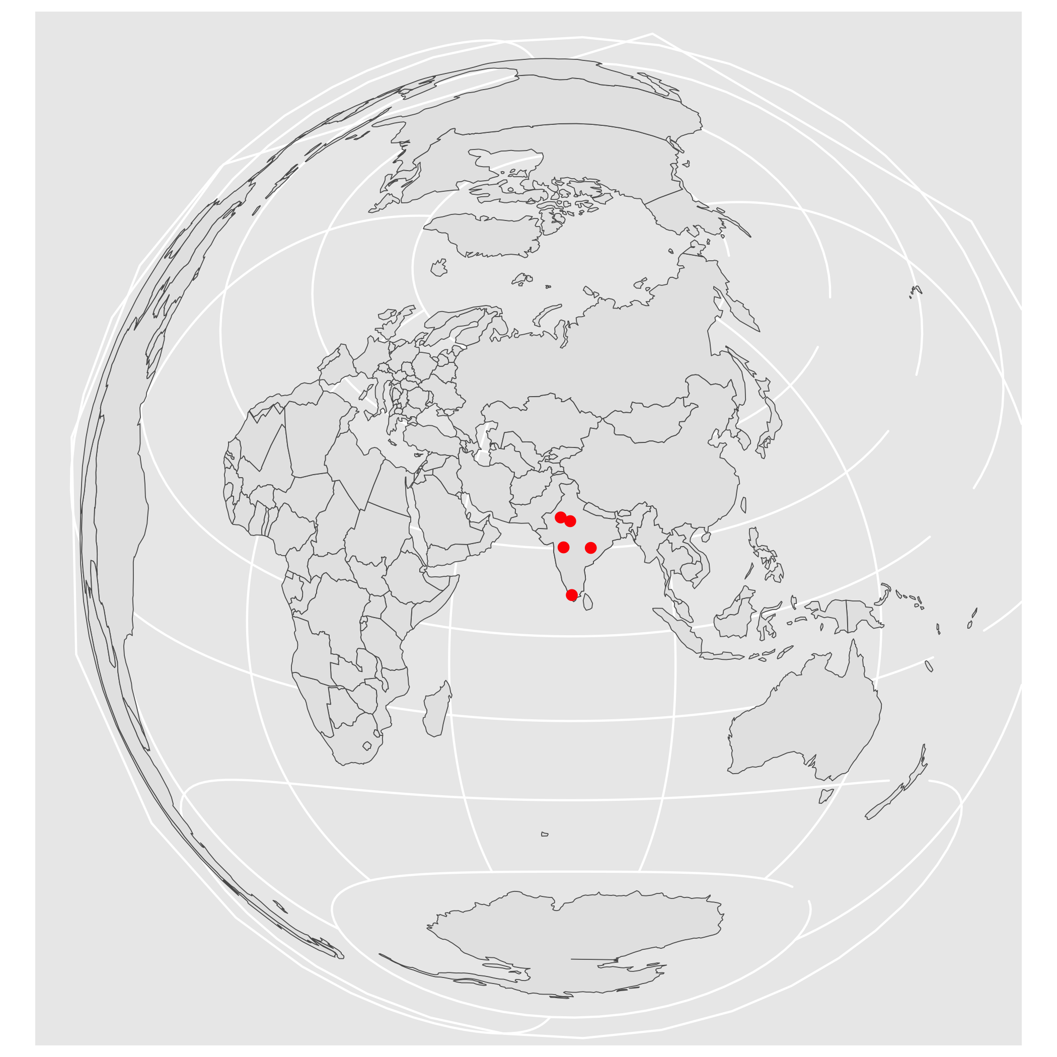
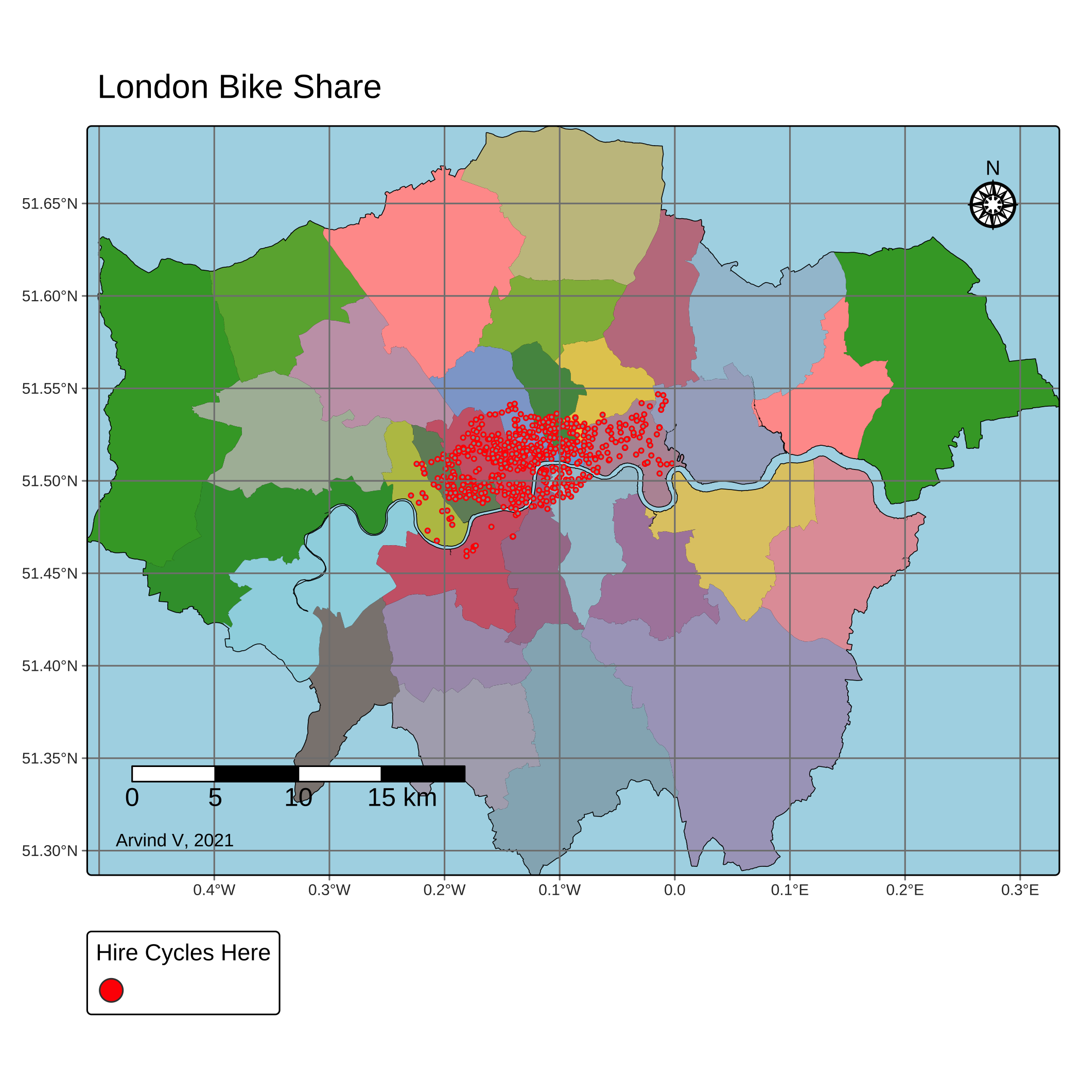
Mapping
tm_shape(lnd) + tm_borders(col = "black", lwd = 1) + tm_fill("NAME", legend.show = FALSE)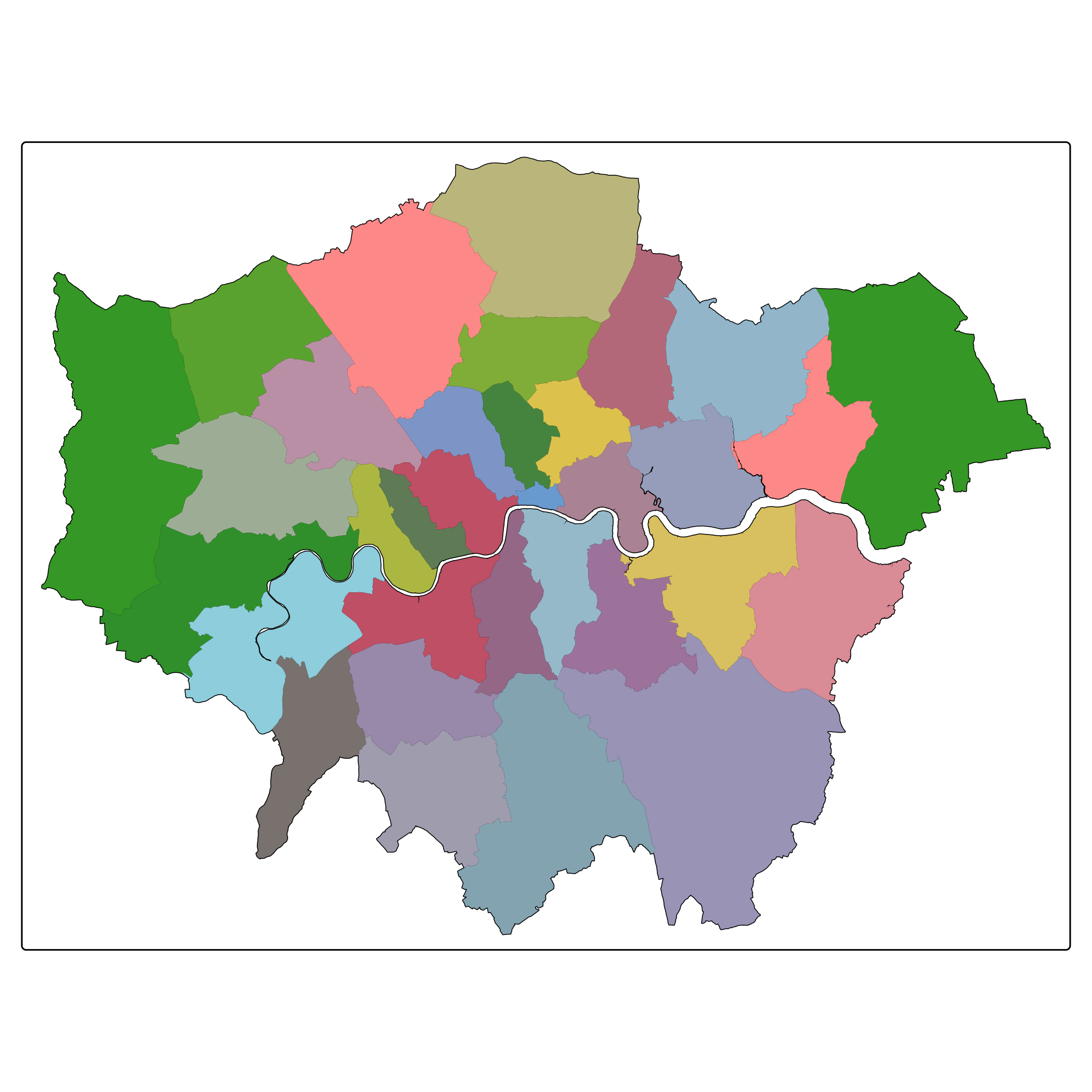
tmap Layers are in groups
Groups start with tm_shape(data = ...)
Groups are "connected" with a sign as usual...
# Group 1tm_shape(lnd) + tm_borders(col = "black",lwd = 1) + tm_fill("NAME", legend.show = FALSE) +# Group 2 = Layer 2 tm_shape(cycle_hire_osm) + tm_symbols(size = 0.2, col = "red")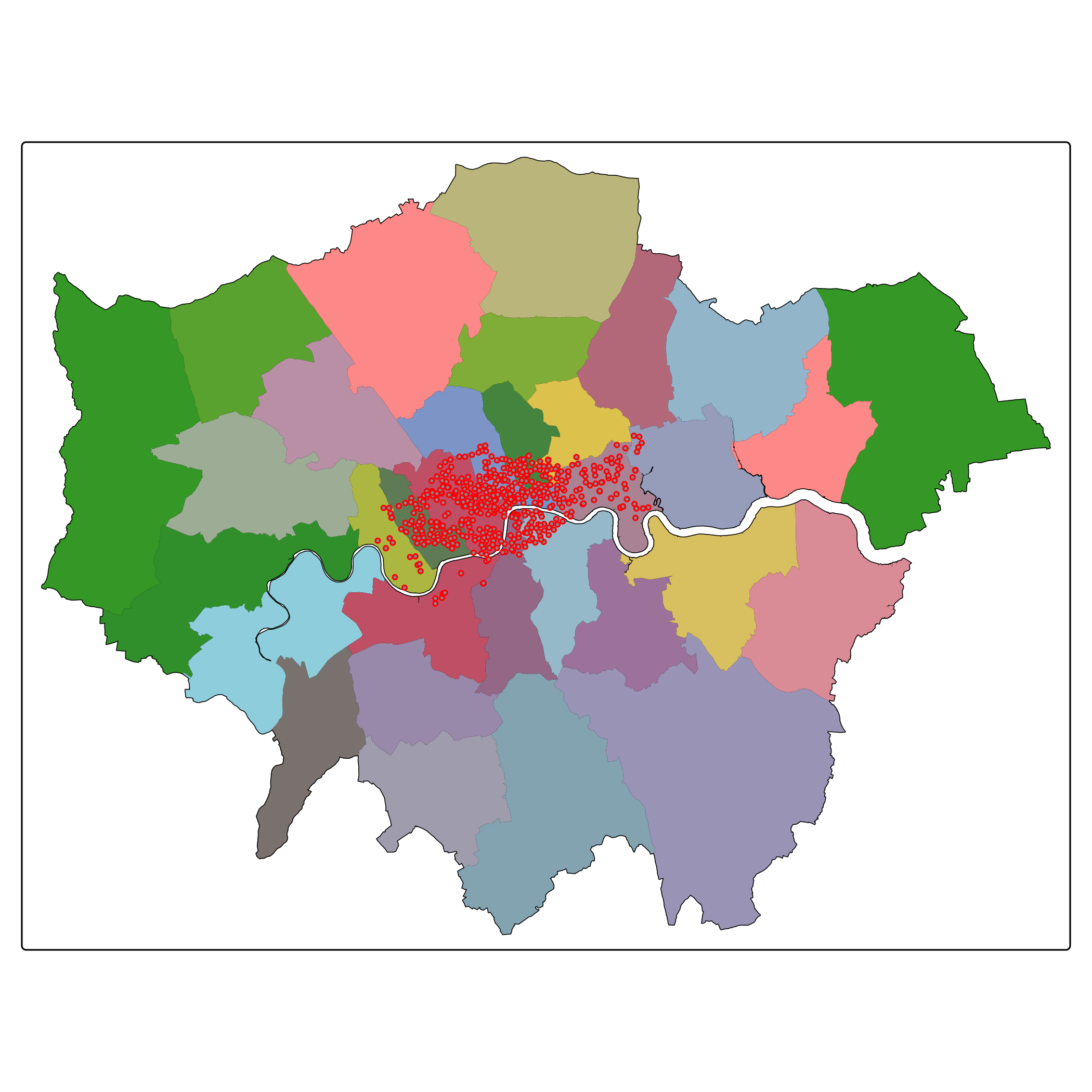
Add graticules and legends
# Group 1tm_shape(lnd) + tm_borders(col = "black",lwd = 1) + tm_fill("NAME", legend.show = FALSE) +# Group 2 = Layer 2 tm_shape(cycle_hire_osm) + tm_symbols(size = 0.2, col = "red") + tm_graticules() + tm_add_legend(type = "symbol", col = "red", title = "Hire Cycles Here")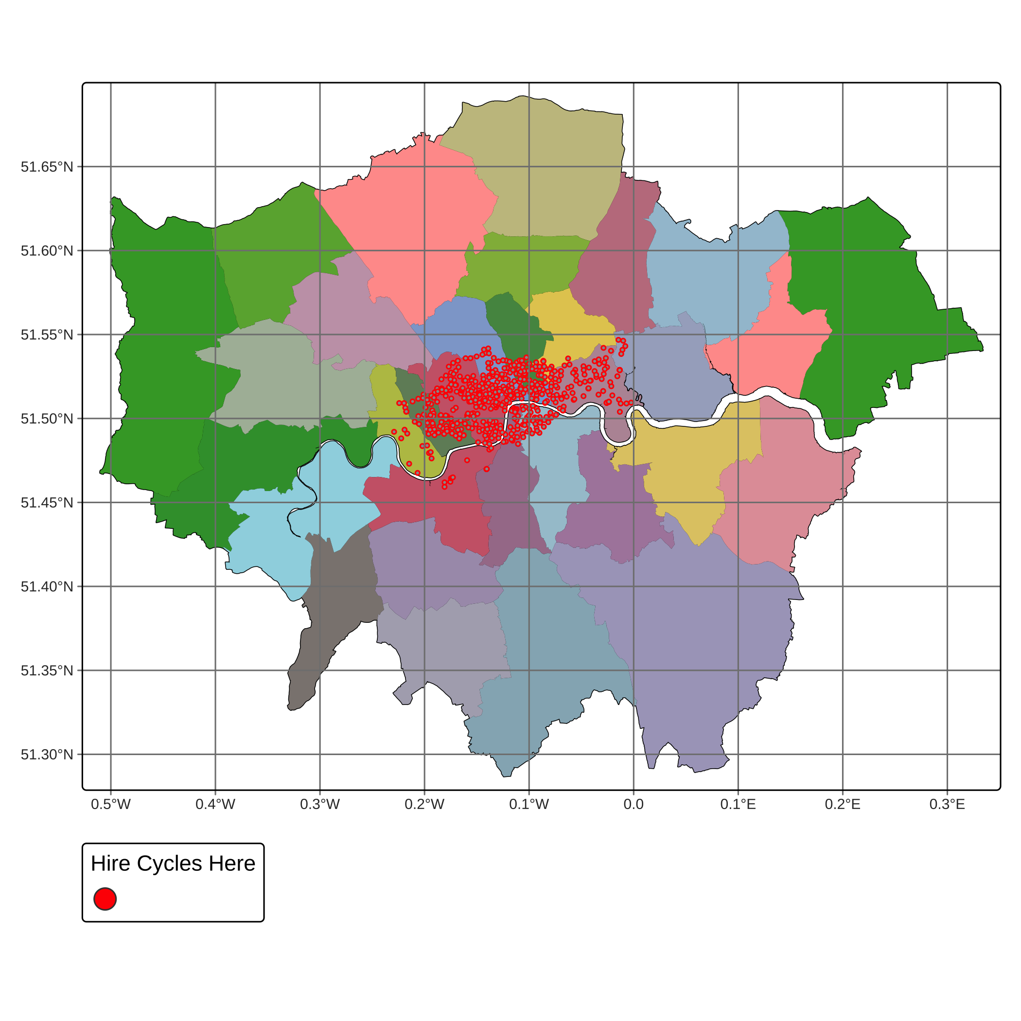
Add Scale and Compass to the Map
# Group 1tm_shape(lnd) + tm_borders(col = "black",lwd = 1) + tm_fill("NAME", legend.show = FALSE) +# Group 2 = Layer 2 tm_shape(cycle_hire_osm) + tm_symbols(size = 0.2, col = "red") + tm_graticules() + tm_add_legend(type = "symbol", col = "red", title = "Hire Cycles Here") + tm_scale_bar(position=c("left", "bottom"), text.size = 1) + tm_compass(position = c("right", "top"), type = "rose", size = 2)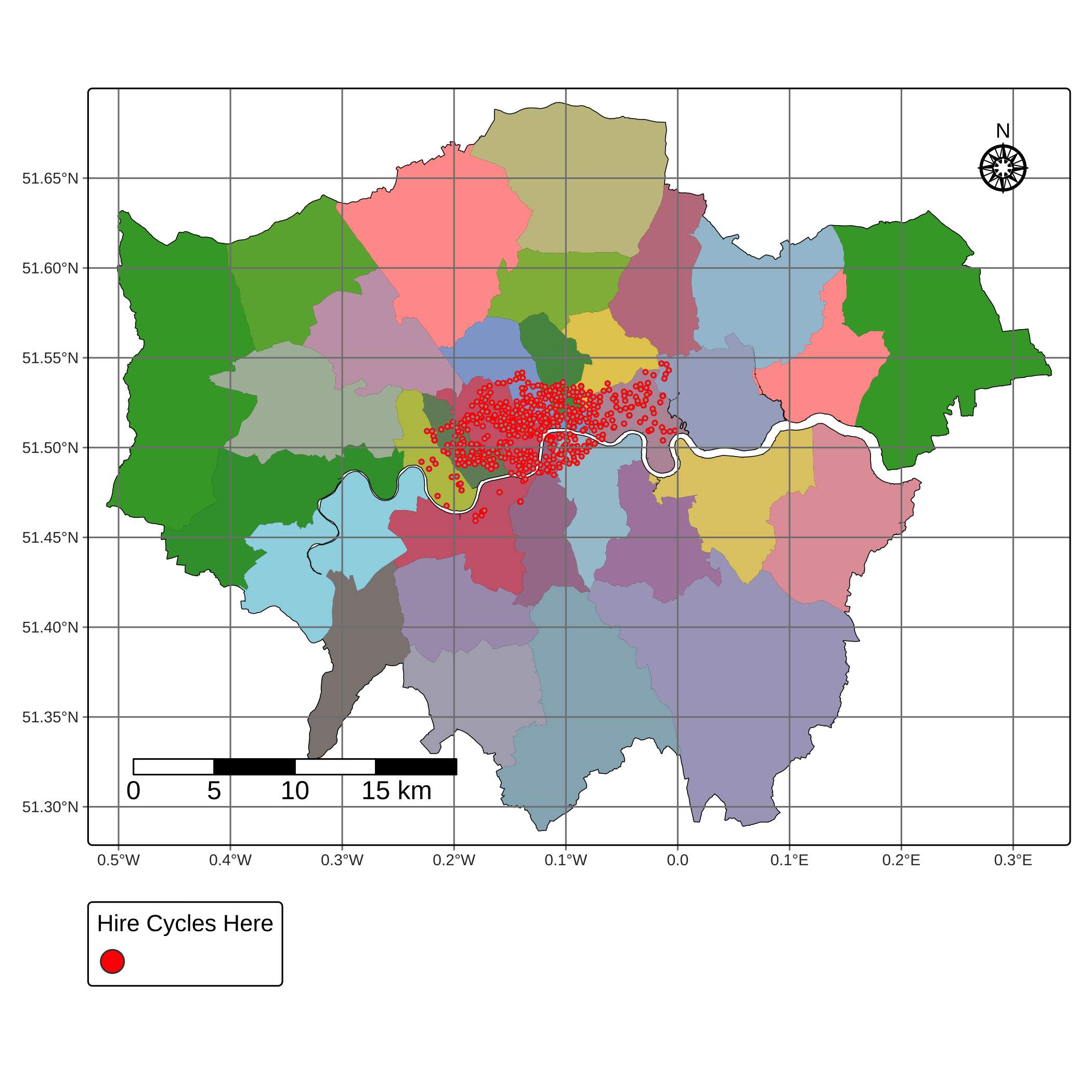
Add Credits and Layout Options
mymap <- tm_shape(lnd) + tm_borders(col = "black", lwd = 1) + tm_fill("NAME", legend.show = FALSE) +tm_shape(cycle_hire_osm) + tm_symbols(size = 0.2, col = "red") + tm_graticules() + tm_add_legend(type = "symbol", col = "red", title = "Hire Cycles Here") + tm_scale_bar(position=c("left", "bottom"),text.size = 1) + tm_compass(position = c("right", "top"), type = "rose", size = 2) + tm_credits(text = "Arvind V, 2021", position = c("left", "bottom")) + tm_layout(main.title = "London Bike Share", bg.color = "lightblue", inner.margins = c(0, 0, 0, 0))mymap